Air quality and health impacts of the 2020 wildfires in California

Abstract

Background

Wildfires in 2020 ravaged California to set the annual record of area burned to date. Clusters of wildfires in Northern California surrounded the Bay Area covering the skies with smoke and raising the air pollutant concentrations to hazardous levels. This study uses the Fire Inventory from the National Center for Atmospheric Research database and the Community Multiscale Air Quality model to estimate the effects of wildfire emissions on air quality during the period from August 16 to October 28 of 2020. In addition, low-cost sensor data for fine particulate matter (PM_2.5) from the PurpleAir network is used to enhance modeled PM_2.5 concentrations. The resulting impacts on ozone and PM_2.5 are used to quantify the health impacts caused by wildfires using the Benefits Mapping and Analysis Program – Community Edition.

Results

Wildfire activity significantly increased direct PM_2.5 emissions and emissions of PM_2.5 and ozone precursors. Direct PM_2.5 emissions surged up to 38 times compared to an average day. Modeling results indicated that wildfires alone led to a rise in ozone daily maximum 8-h average by up to 10 ppb and exceeded PM_2.5 air quality standards in numerous locations by up to 10 times. While modeled PM_2.5 concentrations were lower than measurements, correcting these with PurpleAir data improved the accuracy. The correction using PurpleAir data increased estimates of wildfire-induced mortality due to PM_2.5 exposure by up to 16%.

Conclusions

The increased hospital admissions and premature mortality attributed to wildfires were found to be comparable to the health impacts avoided by strategies aimed at meeting ozone and PM2.5 air quality standards. This suggests that widespread wildfire emissions can negate years of efforts dedicated to controlling air pollution. The integration of low-cost sensor data proved invaluable in refining the estimates of health impacts from PM2.5 resulting from wildfires.

Resumen

Antecedentes

Los incendios de vegetación en 2020 devastaron California, fijando el récord anual de área quemada hasta el presente. Ese año, múltiples grupos de incendios en el norte de California rodeaban el área de la Bahía (Bay Area), cubriendo los cielos de humo y elevando las concentraciones de contaminantes hasta niveles peligrosos. Este estudio usó el Inventario de Incendios de la base de datos del Centro Nacional para Investigaciones de la Atmósfera y del modelo Comunitario Multiescalar sobre la Calidad del Aire, para estimar los efectos de las emisiones de incendios sobre la calidad del aire desde el 16 de agosto hasta el 28 de octubre de 2020. Adicionalmente, el sensor de bajo costo para determinar el particulado fino (PM2.5), tomado de la red PurpleAir, fue usado para mejorar el modelado de concentraciones de PM2.5. Los impactos resultantes en el ozono y PM2.5 fueron usados para cuantificar los impactos en la salud causados por los incendios de vegetación, usando el Programa Beneficios del Mapa y Análisis - Edición de la Comunidad.

Resultados

La actividad de los incendios incrementaron significativamente las emisiones directas de PM2.5 y los precursores de las emisiones de PM2.5 y ozono. Las emisiones directas de PM2.5 resultaron hasta 38 veces más altas comparadas con un día normal. Los resultados modelados indicaron que los incendios por sí mismos llevaron a un aumento del ozono diario máximo 8 horas en promedio y por 10 ppb, y excedieron los estándares de calidad del aire debido al PM2.5 en numerosas ubicaciones y por hasta 10 veces. Mientras que los valores modelados del PM2.5 fueron más bajos que las mediciones, la corrección de esos valores con el PurpleAir mejoraron su exactitud. Las correcciones usando datos de PurpleAir incrementaron las estimaciones de la mortalidad debida a la exposición de PM2.5 en un 16%.

Conclusiones

El incremento en las admisiones en los hospitales y las muertes prematuras atribuidas a los incendios de vegetación fueron encontradas comparables a los impactos en la salud evitados mediante estrategias enfocadas a alcanzar los estándares de calidad del aire para el ozono y el PM2.5. Esto sugiere que las emisiones generalizadas de los incendios pueden anular años de esfuerzos dedicados a controlar la contaminación del aire. La integración de datos del sensor de bajo costo probó ser muy valiosa para refinar las estimaciones de los impactos en la salud provenientes del PM2.5 resultante de los incendios.

Background

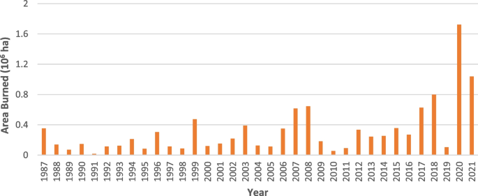
The year 2020 saw the largest area burned due to wildfires in California in recorded history (Fig. 1) and included 5 of the top 7 largest wildfires ever recorded in California. More than 1.7 million hectares burned in 8648 incidents, and 33 people perished as a direct result of the fires (CalFire 2022). The largest fires started in mid-August, clustering across northern California and around the Bay area, which famously turned San Francisco daylight skies into an apocalyptic orange twilight for several days. Because of the large and widespread fires, the state experienced long episodes of elevated fine particulate matter (PM_2.5, i.e., particulate matter with diameter smaller than 2.5 micrometers) concentrations (Li et al., 2021). Exposure to elevated concentrations of PM_2.5 is linked to increased respiratory and cardiovascular illnesses and can lead to increased mortality (Atkinson et al. 2014, Brook et al., 2010).

Fig. 1

Recorded area burned in wildfire events by year in California. (Source: CalFire, 2022)

Prior research has investigated the effects of recent wildfires on air quality and public health through two primary methodologies. One approach involves employing wildfire emissions and chemical transport models to simulate the contribution of wildfires to PM_2.5 levels, as demonstrated by studies conducted by Shi et al. (2019) and Lassman et al. (2023). The other method utilizes direct measurements obtained from ground-based or satellite observations to map pollutant concentrations and subsequently estimates the portion attributed to wildfires, as seen in research by Wang et al. (2021) and Enayati Ahangar et al. (2022).

Shi et al. (2019) specifically examined the impact of wildfires in Southern California in December 2017, utilizing various satellite-based techniques and a chemical transport model to estimate wildfire emissions and their influence on PM_2.5 concentrations and population exposure. Their study revealed that exposure to PM_2.5 induced by wildfires in December accounted for over 40% of the total annual PM_2.5 exposure in certain locations. Lassman et al. (2023) used a chemical transport model to compare two different wildfire emission schemes that are used by the air quality modeling community: the Fire Inventory from the National Center for Atmospheric Research (FINN, Wiedinmyer et al., 2011) and the Surface Fire model (SFIRE, Mandel et al., 2012). Although SFIRE provided a more accurate representation of fire location and timing, the resulting PM_2.5 modeling outcomes were only marginally more accurate than those obtained using FINN when compared to measured values of PM_2.5.

In another study, Wang et al. (2021) utilized a combination of monitoring and satellite data to map PM_2.5 concentrations in California during the latter half of 2018. This research used low-resolution fire emissions and chemical transport models and assessed the direct and indirect economic impacts and capital losses incurred due to wildfire disruptions.

Enayati Ahangar et al. (2022) explored PM_2.5 concentration mapping over California's San Joaquin Valley in late summer and fall of 2020, utilizing regulatory monitors and low-cost sensors from the PurpleAir sensor network (PurpleAir, 2022). PurpleAir sensors use a low-cost technology to estimate concentrations of particulate matter and data is reported in real time to the PurpleAir website. Enayati Ahangar et al. employed a trajectory model to quantify the contribution of wildfires to total PM_2.5 concentrations, utilizing fire emissions estimates derived from satellite observations. Kramer et al. (2023) used data from regulatory monitors and PurpleAir sensors and used various interpolation techniques to estimate exposure to wildfire-induced pollution in Northern and Southern California.

The goal of this study is to estimate the impact of wildfire emissions on air quality and public health in California from mid-August to late October in 2020. The methodology in this study integrates two approaches mentioned above. Specifically, it combines a wildfire emissions inventory and a comprehensive chemical transport model with ground-based observations to gauge the influence of wildfires on air pollution. Ground-based monitoring data are employed to refine the PM_2.5 model estimates, thereby enhancing our understanding of the effects of wildfire emissions on PM_2.5 concentrations and population exposure. Furthermore, the air quality impacts resulting from wildfires are assessed in terms of health using the Benefits Mapping and Analysis Program – Community Edition model (BenMAP-CE, U.S. EPA, 2021).

2020 fire season

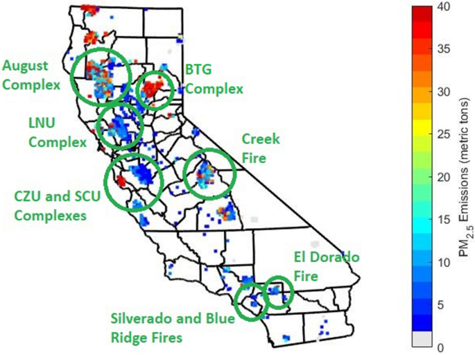
This study focuses on the period between August 16 and October 28, 2020. Initially, this period was marked by a series of wildfires in the northern portion of the state, primarily ignited by lightning strikes. These fires began as small, isolated, and scattered incidents but rapidly evolved into substantial fire complexes that persisted for weeks. The fire complexes, as depicted in Fig. 2, included the August, Sonoma-Lake-Napa Unit (LNU), San Mateo-Santa Cruz Unit (CZU), Santa Clara (SCU), and the Butte/Tehama/Glenn (BTG) lightning complexes. Among these large wildfires, the August complex became the largest wildfire ever recorded in California. In early September, the Creek fire developed quickly in the Sierras producing a large pyrocumulonimbus cloud that reached altitudes of more than 15,000 meters above sea level. Around the same time, the El Dorado fire broke out in Southern California. At the end of October, fanned by strong Santa Ana winds, the Silverado and Blue Ridge fires ignited. In addition to in-state wildfires, large wildfires that originated in Oregon also contributed to air pollution in California, as satellite images (NASA Worldview 2020) showed smoke being transported southwards and reaching the San Francisco Area around mid-September.

Fig. 2

Cumulative PM_2.5 emissions from wildfires during the period August 16–October 28, 2020

Methods

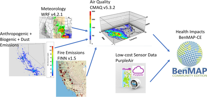
The modeling framework, illustrated in Fig. 3, comprises multiple models designed to estimate different factors and processes related to air pollution formation. These models calculate the resulting impacts on both air quality and public health and are described in more detail in this section. In general terms, the framework includes a meteorological model to assess the weather conditions during the modeling period, models to estimate anthropogenic, biogenic, and wildfire emissions, and a chemical transport model to analyze the formation and transport of air pollutants. Additionally, data from PurpleAir sensors are utilized to assess and refine certain correction methods for air pollution estimates. Finally, a comprehensive model is employed to evaluate the health effects of air pollution induced by wildfires. Specific details on each individual model are described below.

Fig. 3

Diagram of the modeling setup for this study. Emissions and meteorological inputs are used to run the air quality model. Low-cost sensor data is used to analyze potential correction methods, and adjusted results are used to calculate potential health impacts using the health impact model.

The modeling period spanned from August 16 to October 28, 2020. Meteorology fields for the study period were generated using the WRF model, version 4.2.1 (Skamarock et al. 2019). The model was initialized with the National Center for Environmental Prediction Final (NCEP FNL) Operational Global Analysis data (NCEP 2021) and was run in nested mode with two domains: the outer domain at a 12-km grid resolution and the inner domain at a 4-km grid resolution. The model was run in staggered periods of 5 days, with modeling being reinitialized by reanalysis data every 3 days. The first 2 days were used for spin-up, and the remaining 3 days were used for air quality modeling. The following physics options were selected: (1) Purdue Lin scheme microphysics (Chen and Sun 2002), (2) YSU planetary boundary layer (PBL) scheme (Hong, Noh and Dudhia 2006), (3) NOAH land-surface (Campbell et al. 2019), (4) Grell G3D cumulus parameterization (Grell and Devenyi 2002), and (5) Rapid Radiative Transfer Model (RRTM) longwave (Mlawer et al. 1997) with Goddard shortwave radiative transfer schemes (Matsui et al. 2020).

Air quality was modeled using the Community Multiscale Air Quality model (CMAQ, Byun and Schere, 2006), version 5.3.2. Version 5.3.2 includes minor bug fixes with respect to version 5.3.1, which was documented and validated by Appel et al. (2021). Initial and boundary conditions were derived from concentration fields from the Whole Atmosphere Community Climate Model (WACCM) configuration of the Community Earth System Model 2 (CESM2) (Gettelman et al. 2019).

Anthropogenic emissions were derived from the California Air Resources Board’s (CARB) emissions inventory. Area and off-road emissions were spatially resolved using source-specific spatial surrogates developed by CARB. On-road emissions were generated using CARB’s on-road emissions model EMmission FACtor (EMFAC) (EMFAC2017, CARB 2020) and spatially allocated using the Emissions Spatial and Temporal Allocator (ESTA) (CARB 2021). Dust and biogenic emissions were calculated inline in CMAQ. Inline biogenic emissions were based on the Biogenic Emissions Inventory System version 3.61, which used the Biogenic Emissions Land-use Database (version 3) with 1-km resolution (U.S. EPA, 2016).

Fire emissions were developed based on FINN version 1.5 (Wiedinmyer et al. 2011). Fire emissions included trace gas and particle emissions from open burning of biomass, which accounts for wildfires, agricultural fires, and prescribed burning. The emissions were estimated using satellite observations of fire detections and vegetation density from the moderate resolution imaging spectroradiometer (MODIS) instruments, land cover data, and emission factors specific for each type of land use/land cover. Resolution of fire emissions is 1 km, and their chemical speciation was converted to the Statewide Air Pollution Research Center (SAPRC)-07 chemical mechanism. The daily average and daily maximum wildfire emissions during the modeling period are shown in Table 1, along with average and maximum daily anthropogenic emissions. On average, wildfires emitted nitrogen oxides (NO_X) at a comparable rate to that of anthropogenic emissions, whereas reactive organic gas (ROG) emissions from wildfires were more than five times higher than those from anthropogenic sources. NO_X and ROG are precursors to ozone formation and secondary PM_2.5. Wildfires also emitted significantly more PM_2.5 precursors such as sulfur oxides (SO_X) and ammonia (NH₃) than anthropogenic sources. Finally, direct emissions of PM_2.5 from wildfires were nearly nine times larger than those from anthropogenic sources. The day with the highest emissions was September 9, 2020, when the August Complex Fire and the Creek Fire were at their peak. In that day, PM_2.5 emissions from wildfires were 38 times the average emissions from anthropogenic sources. Overall, wildfires contributed severely to air pollutant emissions and impacted the air quality across large areas in the state.

Table 1 California state-wide pollutant emissions from anthropogenic and wildfire emissions. Anthropogenic emissions represent the average daily emissions during the modeling period

The air quality modeling evaluation for ozone and PM_2.5 was based on observations extracted from the Air Quality System (AQS) database. A total of 172 stations measuring ozone and 120 stations measuring PM_2.5 were included in the analysis. The overall model performance is evaluated based on the following statistical parameters: mean bias (MB), mean error (ME), mean normalized bias (MNB), and mean normalized error (MNE). These parameters are defined as follows (Emery et al., 2017):

$$\textrm{MB}=\frac{1}{N}\sum_j\left({P}_j-{O}_j\right)$$

(1)

$$\textrm{ME}=\frac{1}{N}\sum_j\mid {P}_j-{O}_j\mid$$

(2)

$$\textrm{MNB}=\frac{1}{N}\sum_j\frac{\left({P}_j-{O}_j\right)}{O_j}\times 100$$

(3)

$$\textrm{MNE}=\frac{1}{N}\sum_j\frac{\mid {P}_j-{O}_j\mid }{O_j}\times 100$$

(4)

in which P_j denotes model prediction on day j, O_j denotes observed concentration on day j, and N is the total number of observed data points.

This study used data from PurpleAir sensors, which constitute a large network of low-cost monitors that measure particle pollution, to enhance the modeling of PM concentrations. PurpleAir sensors use laser technology to count suspended particles that range from 0.3 to 10 μm. The particle counts are then processed by a complex algorithm to calculate PM₁₀, PM_2.5, and PM_1.0 mass concentration (PurpleAir, 2022). Due to the limitations in low-cost sensor technology, bias in PM concentrations measured by PurpleAir sensors is expected. Previous studies analyzed the performance of PurpleAir sensors collocated with regulatory monitors, and correction factors using ambient meteorological parameters have been proposed. The United States Environment Protection Agency (U.S. EPA) analyzed many complex correction schemes and suggested that a simple linear correction using ambient relative humidity provides a good approximation at a national level (Barkjohn et al. 2021). Shulte et al. (2020) also proposed binning the correction algorithm into two spaces of low and high PM_2.5 concentrations and including seasonality as an additional correction parameter.

This study used data from 5661 outdoor sensors spread throughout California and calculated the correction factors based on daily PM_2.5 observations from 120 reference monitors. Sensors that were within 0.02°radius (~2 km) from regulatory monitors were used to calculate the linear correction parameters following the approach proposed by Barkjohn et al. (2021) and the concentration binning used by Schulte et al. (2020) for two models: one for concentrations below 35 μg/m³ and the other for concentrations equal or above 35 μg/m³.

The linear correction scheme obtained using measurements from the period August 16 to October 28 was as follows:

$$\textrm{For}\ {\textrm{PM}}_{2.5}<35\upmu \textrm{g}/{\textrm{m}}^3,{\textrm{PM}}_{2.5}=0.5225\times \textrm{PA}-0.0768\times \textrm{RH}+7.4352\ {R}^2=0.3938$$

$$\textrm{For}\ {\textrm{PM}}_{2.5}<\frac{35\upmu \textrm{g}}{{\textrm{m}}^3},{\textrm{PM}}_{2.5}=0.7792\times \textrm{PA}+0.0684\times \textrm{RH}-5.8310\kern0.75em {R}^2=0.6886$$

in which PA denotes the PurpleAir PM_2.5 data and RH denotes the relative humidity.

Two approaches were employed to interpolate PurpleAir corrected measurements and to blend them with modeling results: (1) using inverse squared distance weighting for PurpleAir measurements and model gradient adjustment based on the modeled daily PM_2.5 values from the simulation that includes fire emissions and (2) using kriging of the model-to-measured ratios.

Inverse squared distance weighting (ISDW) for PurpleAir measurements with model gradient adjustment

Inverse distance weighting is commonly used as an interpolation method to estimate concentration maps of air pollutants based on monitoring data. For example, inverse distance weighting is used by the Software for Model Attainment Test – Community Edition (SMAT-CE) developed by the U.S. EPA to determine attainment status over unmonitored areas (U.S. EPA, 2022). While the recommended exponent of the inverse distance weights can vary depending on the application (de Mesnard, 2013), the SMAT-CE model uses inverse squared distance weighting as the default option.

In this study, once all the daily PM_2.5 were corrected, daily PM_2.5 concentration maps were generated using interpolated PurpleAir measurements at the 4 km by 4 km grid level using inverse square distance weighting and gradient adjustment based on the modeled daily PM_2.5 values from the simulation that included fire emissions. The PurpleAir sensors used in the interpolation were limited to the ones within a radius of 40 km from each cell centroid. Modeled values were also included as artificial monitors to constrain grid cells that are far from monitors to concentrations informed by the modeled results. The expression used to calculate the Purple Air concentration maps is as follows:

$${C}_{i,\textrm{fires}}=\left({\textrm{Mod}}_{i,\textrm{fires}}+\sum_{k=1}^N\frac{1}{{D_k}^2}{\textrm{PA}}_k\frac{{\textrm{Mod}}_{i,\textrm{fires}}}{{\textrm{Mod}}_{k,\textrm{fires}}}\right)/\left(1+\sum_{k=1}^N\frac{1}{{D_k}^2}\right),$$

(5)

where C_i,fires is PM_2.5 concentration in cell i, D_k is the distance of sensor k to cell i, PA_k is corrected PurpleAir PM_2.5 concentration from sensor k, and Mod_i,fires and Mod_k,fires are the modeled daily PM_2.5 concentration in cell i and at sensor location k, respectively. The distance, D_k, is expressed in terms of discreet cell lengths, where sensors in cell i have D_k=1, and every increment in cell distance is added as integer values.

Kriging of model-to-measured ratios

Kriging is an advanced geostatistical procedure that generates an estimated surface from a scattered set of points by performing a regression that produces a least-squares estimate of the data (Remy et al., 2011). Kriging has been used to interpolate measured pollutant concentrations to determine air pollution exposure (Lassman et al., 2017, Yu et al., 2018, Kramer et al., 2023). Yu et al. (2018) compared various methods of interpolation for air pollution field estimations and suggested the blending of measured and modeled data by using ordinary kriging of the ratios of modeled-to-observed concentrations. We constructed the experimental semivariogram for each individual day with the ratios of modeled daily PM_2.5 over observed daily PM_2.5. We tested three different semivariogram models: spherical, gaussian, and exponential. Based on the sum of the squared of the residuals between the experimental semivariogram and the model, the spherical and gaussian models resulted in the best fit.

Conversely, the estimated concentration maps adjusted to PurpleAir data without the impact of wildfires were calculated as follows:

$${C}_{i,\textrm{nofires}}={C}_{i,\textrm{fires}}\times \frac{{\textrm{Mod}}_{i,\textrm{nofires}}}{{\textrm{Mod}}_{i,\textrm{fires}}},$$

(6)

where C_i,nofires is the PurpleAir-adjusted concentration without the contribution of wildfires in cell i and Mod_i,nofires is the modeled daily PM_2.5 concentration without wildfire emissions in cell i.

BenMAP-CE version 1.5 was used to estimate the increase incidence of health end points due to wildfires (U.S. EPA, 2021). BenMAP-CE converts air pollutant concentration increments into health impacts with the use of concentration-response (C-R) functions. C-R functions are derived from epidemiology studies and provide the relation between a change in pollutant concentration and an increase in the incidence of a given health impact indicator from a baseline incidence rate. Baseline incidence rates for this study are based on values developed in earlier analysis for Southern California (South Coast AQMD 2017a) and later used to determine the health and economic impacts from California fires in 2018 (Wang et al. 2019). Information on the concentration-response functions used in this study are summarized in Table 2 and their respective function forms are described in Table 3. In general, the functions depend on population (P), rate of incidence of a particular health end point (I), change in concentration of a pollutant (ΔC), and fitting parameters A and β. The baseline function represents the reference value of incidence of a particular health end point (e.g., hospital admission, death) with a zero change in air pollutant concentrations. The concentration-response function calculates an increase in incidence of a particular health end point due to a change in pollutant concentration (ΔC).

Table 2 Concentration response functions used to quantify health impacts. Function forms shown in Table 3

Table 3 Forms of the concentration-response functions and the baseline functions to calculate health impacts as a function of change in pollutant concentration (ΔC), incidence rate (I), population (P), and fitting coefficients A and β

Results

Air quality modeling results and model performance

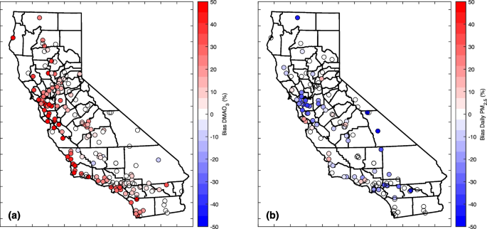
Model performance is presented in Table 4. The model overestimated ozone concentrations, most notably along coastal stations, with better performance in stations in the eastern portion of the Los Angeles Basin and in the Central Valley, where ozone concentrations are typically the highest (Fig. 4a). Generally, PM_2.5 concentrations were underpredicted throughout the state, in part possibly due to the model inability to capture fully the effects of wildfires. As shown in Fig. 4b, the largest PM_2.5 underpredictions occurred east of the San Francisco Bay Area, which was highly impacted by wildfire smoke throughout the wildfire season.

Table 4 Overall air quality modeling performance for O₃ and PM_2.5

Fig. 4

Mean normalized bias (MNB) during the modeling period for a daily maximum 8-h ozone (DMAO₃) and b daily PM_2.5. Values are normalized with observations, as described in Eqs. 3–4.

Results presented in this study for PM_2.5 are consistent with the negative biases reported for CMAQ version 5.3.1 for California (Appel et al., 2021). Appel et al. (2021) reported model performance of CMAQ version 5.3.1 for the continental US in 2016 at 12 km resolution. Although in 2016 only moderate wildfire activity was recorded in California, the model performance was characterized by biases contained between +4% and −8% for ozone and consistently negative and as low as −30% for PM_2.5, like the biases shown in the present study. It is also likely that the exceptionally high wildfire activity recorded during the modeling period considered in this study may have negatively affected CMAQ’s ability to reproduce observed PM_2.5 concentrations.

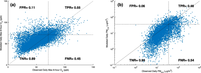
An alternate method to evaluate model performance is to determine the model capability to predict exceedances with respect to U.S. EPA’s national ambient air quality standards (NAAQS). Fig. 5 presents scatter plots of modeled versus observed concentrations for daily maximum 8-h ozone and daily PM_2.5. The lines indicating each respective standard delineate four quadrants that define the model fitness to predict exceedances. Each subfigure in Fig. 5 shows from top right and clockwise: true positive, false negative, true negative, and false positive. The true positive rate (TPR) is the ability of the model to detect exceedances compared to observations. Conversely, the true negative rate (TNR) is the ability of the model to detect concentrations below the standard. The false negative rate (FNR) and the false positive rate (FPR) are the complementary values of TPR and TNR, respectively. In general, the model performed better when predicting exceedances for ozone, with TPR = 55%, than for PM_2.5, with TPR = 46%, in part because the model showed a positive bias for ozone and a negative bias for PM_2.5.

Fig. 5

Comparison of observations and modeled concentrations for a daily maximum 8-h average of ozone and b daily average PM_2.5. Diagonal shows the 1:1 modeled vs. observed ratio, and the vertical and horizontal lines show the National Ambient Air Quality Standards level for daily maximum 8-h average of ozone (70 ppb) and daily average PM_2.5 (35 μg/m³). The true positive rate (TPR) is the ability of the model to detect exceedances compared to observations. The true negative rate (TNR) is the ability of the model to detect concentrations below the standard. The false negative rate (FNR) and the false positive rate (FPR) are the complementary values of TPR and TNR, respectively.

Contribution of wildfire emissions to air pollution

An additional air quality model simulation without including wildfire emissions was conducted for the same period between August 16 and October 28, 2020, to quantify the impact of wildfires on ozone and PM_2.5. Figure 6 shows the overall increase in daily maximum 8-h ozone and daily PM_2.5 attributed to wildfire emissions during the modeling period and the relative increase with respect to the simulation without wildfire emissions. The impact of wildfires was localized over the northern half of the state, near the location of the wildfires in Northern California. On average, daily maximum 8-h ozone concentrations increased by up to 10 ppb, and many of the largest increases occurred in areas where ozone concentrations are typically high. In relative terms, daily maximum 8-h ozone concentrations increased on average by up to 20% in some northern California locations. Some stations experienced increases in daily maximum 8-h ozone of over 70 ppb in the third week of August, which suggests that wildfire emissions alone led to exceeding the ozone standard. On average, the daily PM_2.5 concentration increased by up to 39 μg/m³, which for some stations represented an increase of more than 400% over normal average values. For instance, some stations experienced increases of over 350 μg/m³ during the third week of August. Thus, considering that the NAAQS for daily PM_2.5 is 35 μg/m³, on average, many stations exceeded the daily PM_2.5 due to wildfire emissions alone, and stations experienced daily PM_2.5 over ten times higher than the daily PM_2.5 standard during several days.

Fig. 6

Overall contribution of wildfires during the modeling period to a increase in daily maximum 8-h ozone (DMAO₃), b increase in daily PM_2.5, c percentage increase in DMAO₃, and d percentage increase in daily PM_2.5 with respect to the case without fires.

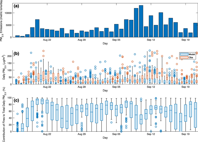
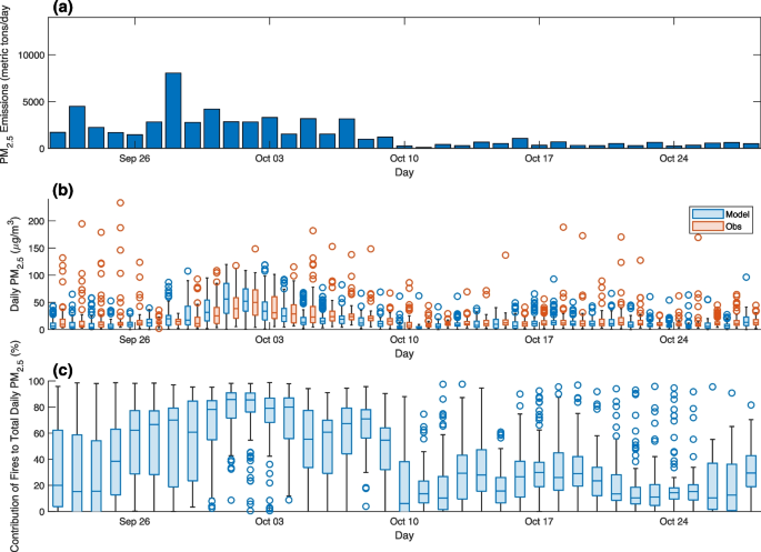
Figures 7 and 8 show the daily variation in PM_2.5 emissions, the observed and modeled daily PM_2.5 concentrations, and daily contribution of fires to total daily PM_2.5 for the periods of August 16–September 21 and September 22–October 28, respectively. PM_2.5 concentrations were particularly underpredicted during the period of September 10–16, trailing the days with the highest emission increases due to wildfires. In addition, based on satellite images, that period was affected by wildfire smoke that originated from wildfires in Oregon, which were not included in the modeling setup. As a result, the impact from wildfire emissions is believed to be underrepresented in the second week of September, and overall, modeling results suggest that the effects of wildfires on daily PM_2.5 presented here are underpredicted.

Fig. 7

Contribution of fires to daily PM_2.5 by day (August 16–September 21): a total daily PM_2.5 emissions from wildfires from FINN, b observed and modeled daily PM_2.5 concentrations, and c modeled contribution of fires to total daily PM_2.5. Whisker/box plot shows the minimum, 1st quartile, median, 3rd quartile, and maximum. Markers show outliers, which are defined as points that are more than 1.5 times the interquartile range (IQR, namely the height of the box) away from the top or bottom of the box.

Fig. 8

Contribution of fires to daily PM2.5 by day (September 22–October 28): a total daily PM_2.5 emissions from wildfires from FINN, b observed and modeled daily PM_2.5 concentrations, and c modeled contribution of fires to total daily PM_2.5. Whisker/box plot shows the minimum, 1st quartile, median, 3rd quartile, and maximum. Markers show outliers, which are defined as points that are more than 1.5 times the interquartile range (IQR, namely the height of the box) away from the top or bottom of the box.

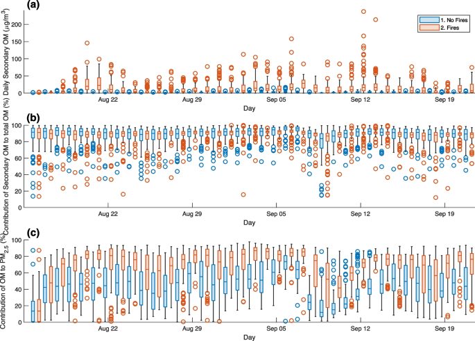
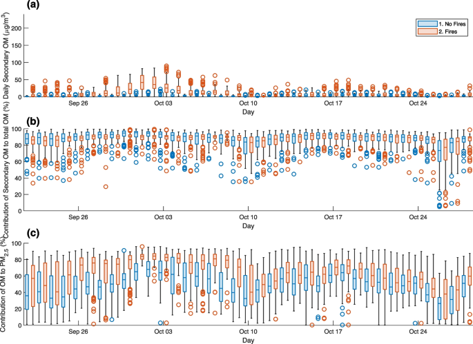
Biomass burning modeled in this study is a major source of atmospheric organic aerosol, typically referred to as brown carbon. Wildfires and brown carbon contribute to the planetary radiative balance and to the formation of secondary organic aerosol, although there are still model limitations in our understanding of the atmospheric transformations of brown carbon (Wong et al. 2019). Figures 9 and 10 present modeled daily concentrations of organic matter (OM) with and without the contribution from wildfires for the periods of August 16–September 21 and September 22–October 28, respectively. They also show that, on average, secondary OM corresponds to more than 90% of the total OM, although the percentage of secondary OM in wildfire-driven OM is slightly smaller than that without the presence of fires because of the large contribution from direct OM emissions. Overall, results suggest that wildfires more than doubled the fraction of OM in aerosol, and the overall OM contribution to total PM_2.5 during fire events was over 80%.

Fig. 9

Comparison of daily OM concentrations without and with the contribution of wildfires (August 16–September 21): a modeled daily average secondary organic aerosol concentrations, b modeled contribution of secondary organic aerosol to total OM, and c modeled contribution of OM to total PM_2.5. Whisker/box plot shows the minimum, 1st quartile, median, 3rd quartile, and maximum. Markers show outliers, which are defined as points that are more than 1.5 times the IQR away from the top or bottom of the box.

Fig. 10

Comparison of daily OM concentrations without and with the contribution of wildfires (September 22–October 28): a modeled daily average secondary organic aerosol concentrations, b modeled contribution of secondary organic aerosol to total OM, and c modeled contribution of OM to total PM2.5. Whisker/box plot shows the minimum, 1st quartile, median, 3rd quartile, and maximum. Markers show outliers, which are defined as points that are more than 1.5 times the IQR away from the top or bottom of the box.

Enhancement of PM2.5 modeling with low-cost sensor data (PurpleAir)

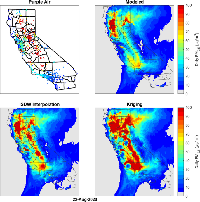
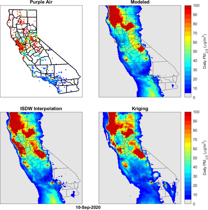
The use of PurpleAir adjustment improved model performance with respect to observations. Pure modeling results have an R² value of 0.27 with respect to PurpleAir observations, whereas the R² values for ISDW and ordinary kriging with a spherical model are 0.74 and 0.76, respectively. Even though the gaussian model for kriging showed similar fitting to the experimental semivariogram, the R² for the modeled adjusted values was less than 0.2. Consequently, ISDW and ordinary kriging with a spherical model, in addition to direct model outputs, were used to determine the health impacts from wildfires during the period of study.

Figures 11 and 12 show two samples of PurpleAir-adjusted daily PM_2.5 concentration fields for two high PM_2.5 events on August 22 and September 10, respectively. In general, PurpleAir-adjusted concentrations were higher than unadjusted model output concentrations. As shown in Fig. 7, the model grossly underestimated PM_2.5 in those events, and thus, the use of PurpleAir correction reduced substantially the negative bias of the modeled PM_2.5.

Fig. 11

Example of PurpleAir-adjusted daily PM_2.5 concentrations on August 22, 2020: measured PurpleAir concentrations (top left), modeled concentrations (top right), PurpleAir-corrected model concentrations using ISDW interpolation (bottom left), and PurpleAir-corrected model concentrations using kriging (bottom right).

Fig. 12

Example of PurpleAir-adjusted daily PM_2.5 concentrations on September 10, 2020: measured PurpleAir concentrations (top left), modeled concentrations (top right), PurpleAir-corrected model concentrations using ISDW interpolation (bottom left), and PurpleAir-corrected model concentrations using kriging (bottom right).

Health impacts

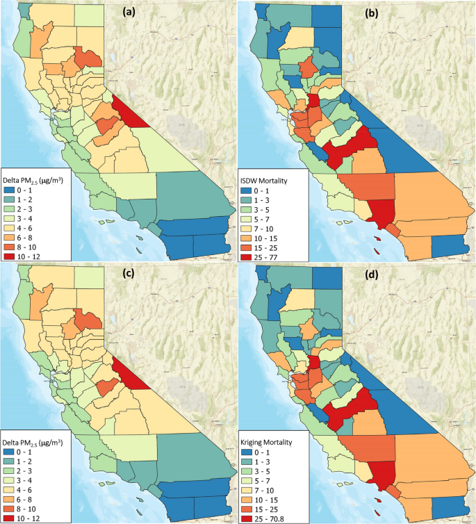
Table 5 shows the health impacts related to increase in ozone and PM_2.5 concentrations resulting from wildfires. PM_2.5 impacts were calculated using both direct model outputs and PurpleAir-adjusted PM_2.5 concentrations. While ozone contributed to increased hospital admissions and mortality, PM_2.5 is the major pollutant of concern regarding health effects. Using unadjusted model data, wildfires caused an additional 1391 hospitalizations and 466 deaths. While these figures constitute a small fraction of California’s total hospitalizations and deaths, it is important to note that annual air pollution-related deaths in the state are estimated at around 40,000 (Wang et al., 2019). Consequently, wildfire-induced pollution estimated in this study accounts for a 1% rise in air pollution-related mortality. However, as discussed before, due to the negative bias of the air quality model with respect to PM_2.5, health impacts using direct model output likely represent an underestimation of the wildfire impacts. The correction using ISDW of PurpleAir data increased the estimated hospital admissions by 35% and the estimated increased deaths by 16%, whereas the correction using kriging of model/PurpleAir ratios increased the estimated hospital admissions by 10% and estimated deaths by 9%. Since air quality models tend to show negative bias for PM_2.5, as reported by Appel et al. (2021) and previously discussed, the use of monitor-based corrections implemented in this study potentially improves the estimates of air quality and health impacts. Given that the performance of ISDW and kriging are very similar, health impact estimates from both methods are considered comparable within the uncertainty bounds.

Table 5 Increase in incidence of major health impacts due to wildfire air pollution (units are in number of admissions, work loss days, and mortality events). Baseline incidence also included for reference.

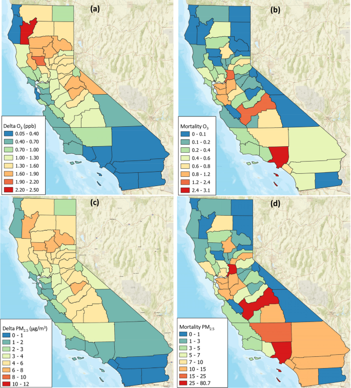
Distribution of health impacts was skewed towards counties with the largest population density, as shown in Fig. 13. In previous studies, it was shown that higher PM_2.5 concentrations during the 2020 California wildfire season were also positively correlated with poverty and housing inequities (Kramer et al. 2023). While the largest fires occurred in the northern half of the state, the highest mortality was estimated to occur in Los Angeles County, which suffered a moderate impact from wildfires but houses one fourth of the state’s population. Figure 14 shows the impacts of PM_2.5 using PurpleAir-adjusted concentrations. Estimated county-level average changes in PM_2.5 increased over the northern half of the state, whereas the incidence of mortality increased the most over the Central Valley.

Fig. 13

Overall impacts of wildfires on air quality and mortality by county using direct modeling results: a average increase in daily maximum 8-h average of ozone, b increased mortality due to ozone increase, c average increase in daily average of PM_2.5, and d increased mortality due to PM_2.5 increase.

Fig. 14

Overall impacts of wildfires using PM_2.5 adjusted with PurpleAir data on air quality and mortality by county: a average increase in daily average of PM_2.5 using ISDW, b average mortality due to PM_2.5 increase using ISDW, c average increase in daily average of PM_2.5 using kriging, and d average mortality due to PM_2.5 increase using kriging.

Discussion and limitations

The increase in hospital admissions due to wildfires is comparable to the potential health impacts of air pollution in the South Coast Air Basin of California (SoCAB), which houses 17 million people out of the total 40 million in California. It is estimated that the drastic emission reductions needed to attain the ozone and PM_2.5 NAAQS in the SoCAB (South Coast AQMD 2017b) would reduce the number of hospital admission by numbers similar to those corresponding to the increase due to wildfire emissions during the modeling period for 2020. Also, the impact of wildfires on premature deaths due to air pollution significantly offsets the premature deaths avoided by the drastic air pollution control strategies that are needed to attain the ozone and PM_2.5 NAAQS.

This study is based on wildfire emissions from the FINN database, which estimates daily emissions from satellite products that include MODIS fire detection and land cover classification. Dispersion and transport of air pollutants and smoke from fires is driven by meteorology, whereas secondary formation of air pollutants—ozone and secondary PM_2.5—depend on atmospheric physicochemical processes that transform primary pollutants. Hence, the results presented in this study depend on the ability of the used models to represent fire emissions, meteorology, and atmospheric chemistry. Moreover, this study demonstrates the use of low-cost sensor data as correction for the negative bias that the air quality model typically displays for PM_2.5 concentrations.

FINN database includes information of daily emissions and starting time of the fire but does not include hourly variation of emissions. For this study, emissions were assumed to be at a daily constant rate since the start of the fire; however, this assumption may misrepresent how emissions interact with background air pollutants that follow a diurnal pattern. Alternative approaches are documented for cases in which FINN fire emissions are adjusted to follow a diurnal profile with minimum emissions at night and peak emissions in the early afternoon (Lassman et al., 2023).

The chemical transport model used in this study, CMAQ, does not include feedback effects of wildfire smoke to meteorology. Studies using chemical transport models that account for feedback effects of PM on the radiative balance, planetary boundary layer height, and temperature have documented decreases in temperature of 1–4 K and decreases in PBL height of 50–400 m (Jiang et al. 2012, Sharma et al., 2022). Lower temperatures can slow down the production of ozone whereas shallow PBL height can enhance the concentration of air pollutants. Also, smoke reduces the downward solar radiation, which reduces the isoprene biogenic emissions and lowers the photolysis rates, and in turn can reduce the formation of ozone and secondary aerosol formation. Lassman et al. (2023) also quantified the effect of wildfires on wind speed and showed that the California wildfires in 2020 reduced wind speed, possibly contributing to slightly less ventilation and higher air pollutant accumulation than the results presented in this study suggest.

Conclusions

This study examines various modeling approaches for assessing the effects of wildfire emissions on ozone and PM2.5 between August 16 and October 28, 2020, a period marked by unprecedented wildfires in California. The research utilizes the FINN database in conjunction with the CMAQ model to estimate the impact of wildfire emissions on air quality. Additionally, the BenMAP-CE model is employed to evaluate the health consequences of air pollution resulting from wildfires.

To address certain limitations in the modeling setup for predicting PM_2.5 concentrations, PurpleAir data was incorporated. The findings indicate that the typically observed negative bias in PM_2.5 displayed by CMAQ is reduced by PurpleAir observations. This reduction in negative bias improves the capability to assess air quality and health impacts related to wildfires. Namely, the study reveals that incorporating PurpleAir data using two distinct methods increases the estimated health impacts of wildfires, resulting in a 9–16% rise in estimated wildfire-induced mortality.

The study observes that California wildfires significantly contributed to elevated levels of ozone and PM_2.5, with an average increase of 2.5 ppb in daily maximum 8-h ozone and an average increase of 12 μg/m³ in daily PM2.5 concentrations. These increases are anticipated to lead to a higher incidence of air pollution-related hospitalizations and premature deaths, potentially causing up to 1886 additional hospitalizations and 539 extra premature deaths. Some of the health impacts stemming from the fires are comparable to the benefits gained from long-term air pollution control strategies designed to meet ozone and PM_2.5 air quality standards. Given the escalating frequency of wildfire events driven by climate change, the health benefits derived from reducing anthropogenic emissions are at times offset by wildfire impacts in the state. The incorporation of low-cost sensor data can enhance the predictive capabilities of air quality models during wildfire events, particularly when these models tend to underestimate particle pollution formation on their own.

References

Appel, K.W., J.O. Bash, K.M. Fahey, K.M. Foley, R.C. Gilliam, C. Hogrefe, W.T. Hutzell, D. Kang, R. Mathur, B.N. Murphy, S.L. Napelenok, C.G. Nolte, J.E. Pleim, G.A. Pouliot, H.O.T. Pye, L. Ran, S.J. Roselle, G. Sarwar, D.B. Schwede, F.I. Sidi, T.L. Spero, and D.C. Wong. 2021. The Community Multiscale Air Quality (CMAQ) model versions 5.3 and 5.3.1: system updates and evaluation. Geoscientific Model Development 14: 2867–2897. https://doi.org/10.5194/gmd-14-2867-2021.
Atkinson, R.W., S. Kang, H.R. Anderson, I.C. Mills, and H.A. Walton. 2014. Epidemiological time series studies of PM2.5 and daily mortality and hospital admissions: a systematic review and meta-analysis. Thorax 69: 660–665.
Barkjohn, K.K., B. Gantt, and A.L. Clements. 2021. Development and application of a United States-wide correction for PM2.5 data collected with the PurpleAir sensor. Atmospheric Measurement Techniques 14: 4617–4637. https://doi.org/10.5194/amt-14-4617-2021.
Bell, M.L., F. Dominici, and J.M. Samet. 2005. A meta-analysis of time-series studies of ozone and mortality with comparison to the national morbidity, mortality, and air pollution study. Epidemiology 16 (4): 436–445.
Brook, R.D., S. Rajagopalan, C.A. Pope III, et al. 2010. Particulate matter air pollution and cardiovascular disease, an update to the scientific statement from the American Heart Association. Circulation 121: 2331–2378.
Byun, D., and K.L. Schere. 2006. Review of the governing equations, computational algorithms, and other components of the Models-3 Community Multiscale Air Quality (CMAQ) modeling system. Applied Mechanics Reviews 59 (2): 51–77.
CalFire, 2022. Cal fire incidents reports. Available at: http://fire.ca.gov/incidents/. Last accessed: May 2022.
Campbell, P.C., J.O. Bash, and T.L. Spero. 2019. Updates to the Noah Land Surface Model in WRF-CMAQ to improve simulated meteorology, air quality, and deposition. Journal of Advances in Modeling Earth Systems 11: 231–256.
CARB 2020, California Air Resources Board EMFAC2017 v 1.0.3 on-road emissions model. Release of latest version of version of EMFAC2017. Available at: https://ww2.arb.ca.gov/our-work/programs/mobile-source-emissions-inventory/msei-modeling-tools-emfac-software-and. Last accessed: May 2022.
CARB 2021, California Air Resources Board Emissions Spatial and Temporal Allocator (ESTA) model. Available at: https://github.com/mmb-carb/ESTA. Last accessed: May 2022.
Chen, S.-H., and W.-Y. Sun. 2002. A one-dimensional time dependent cloud model. Journal of the Meteorological Society of JapanSer. II 80: 99–118.
De Mesnard, L. 2013. Pollution models and inverse distance weighting: some critical remarks. Computers and Geosciences 52: 459–469.
Emery, C., Z. Liu, A.G. Russell, M.T. Odman, G. Yarwood, and N. Kumar. 2017. Recommendations on statistics and benchmarks to assess photochemical model performance. Journal of the Air & Waste Management Association 67 (5): 582–598. https://doi.org/10.1080/10962247.2016.1265027.
Enayati Ahangar F, Cobian-Iñiguez J, Cisneros R. 2022. Combining regulatory instruments and low-cost sensors to quantify the effects of 2020 California wildfires on PM2.5 in San Joaquin valley. Fire 5(3): 64. https://doi.org/10.3390/fire5030064
Gettelman, A., M.J. Mills, D.E. Kinnison, R.R. Garcia, A.K. Smith, D.R. Marsh, S. Tilmes, F. Vitt, C.G. Bardeen, J. McInerny, H.-L. Liu, S.C. Solomon, L.M. Polvani, L.K. Emmons, J.-F. Lamarque, J.H. Richter, A.S. Glanville, J.T. Bacmeister, A.S. Phillips, R.B. Neale, I.R. Simpson, A.K. DuVivier, A. Hodzic, and W.J. Randel. 2019. The Whole Atmosphere Community Climate Model version 6 (WACCM6). Journal of Geophysical Research Atmospheres 124: 12380–12403.
Grell, G.A., and D. Devenyi. 2002. A generalized approach to parameterizing convection combining ensemble and data assimilation techniques. Geophysical Research Letters 29: 38-1–38-4.
Hong, S.Y., Y. Noh, and J. Dudhia. 2006. A new vertical diffusion package with an explicit treatment of entrainment processes. Monthly Weather Review 134: 2318–2341.
Jiang, X., C. Wiedinmyer, and A.G. Carlton. 2012. Aerosols from fires: an examination of the effects on ozone photochemistry in the Western United States. Environmental Science and Technology 46: 442–460. https://doi.org/10.1021/es301541k.
Katsouyanni, K., J.M. Samet, H.R. Anderson, R. Atkinson, A.L. Tertre, S. Medina, et al. 2009. Air pollution and health: a European and North American Approach (APHENA). Research Report (Health Effects Institute).
Kramer, A.L., J. Liu, L. Li, R. Connolly, M. Barbato, and Y. Zhu. 2023. Environmental justice analysis of wildfire-related PM2.5 exposure using low-cost sensors in California. Science of the Total Environment 856 (Part 2): 159218. https://doi.org/10.1016/j.scitotenv.2022.159218.
Lassman, W., B. Ford, R.W. Gan, G. Pfister, S. Magzamen, E.V. Fischer, and J.R. Pierce. 2017. Spatial and temporal estimates of population exposure to wildfire smoke during the Washington state 2012 wildfire season using blended model, satellite, and in situ data. GeoHealth 1: 106–121.
Lassman, W., J.D. Mirocha, R.S. Arthur, A.K. Kochanski, A. Farguell Caus, A.M. Bagley, M. Carreras-Sospedra, D. Dabdub, and M. Barbato. 2023. Using satellite-derived fire arrival times for coupled wildfire-air quality simulations at regional scales of the 2020 California wildfire season. Journal of Geophysical Research: Atmospheres 128 (6): e2022JD037062. https://doi.org/10.1029/2022JD037062.
Li, Y., D. Tong, S. Ma, X. Zhang, S. Kondragunta, F. Li, and R. Saylor. 2021. Dominance of wildfires impact on air quality exceedances during the 2020 record-breaking wildfire season in the United States. Geophysical Research Letters, 48 (21): e2021GL094908. https://doi.org/10.1029/2021GL094908.
Mandel, J., J.D. Beezley, and A.K. Kochanski. 2012. Coupled atmosphere-wildland fire modeling with WRF 3.3 and SFIRE 2011. Geoscientific Model Development 4: 591–610. https://doi.org/10.5194/gmd-4-591-2011.
Matsui, T., S.Q. Zhang, W.-K. Tao, S. Lang, C. Ichoku, and C. Peters-Lidard. 2020. Impact of radiation frequency, precipitation radiative forcing, and radiation column aggregation on convection-permitting West African monsoon simulations. Climate Dynamics 55: 193–213. https://doi.org/10.1007/s00382-018-4187-2.
Mlawer, E.J., S.J. Taubman, P.D. Brown, M.J. Iacono, and S.A. Clough. 1997. Radiative transfer for inhomogeneous atmospheres: RRTM, a validated correlated-k model for the longwave. Journal of Geophysical Research 102: 16663.
Moolgavkar, S.H. 2000. Air pollution and hospital admissions for chronic obstructive pulmonary disease in three metropolitan areas in the United States. Inhalation Toxicology 12 (Supplement 4): 75–90.
Moolgavkar, S.H. 2003. Air pollution and daily deaths and hospital admissions in Los Angeles and Cook counties. In Revised Analyses of Time-Series Studies of Air Pollution and Health. 2003, 183–198. Boston, MA: Health Effects Institute.
Moore, K., R. Neugebauer, F. Lurmann, J. Hall, V. Brajer, S. Alcorn, and I. Tager. 2008. Ambient ozone concentrations cause increased hospitalizations for asthma in children: an 18-year study in southern California. Children's Health Research 116 (8): 1063–1070.
NASA Worldview, 2020. Imagery from the NASA Worldview application, part of the NASA Earth Observing System Data and Information System (EOSDIS). Available at: https://worldview.earthdata.nasa.gov. Last Accessed: November 2022.
NCEP, 2021. National Centers for Environmental Prediction/National Weather Service/NOAA/U.S. Department of Commerce (2000), NCEP FNL Operational Model Global Tropospheric Analyses, continuing from July 1999, /10.5065/D6M043C6, Research Data Archive at the National Center for Atmospheric Research, Computational and Information Systems Laboratory, Boulder, Colo. (Updated daily.) Accessed September 2021.
Ostro, B.D. 1987. Air pollution and morbidity revisited: a specification test. Journal of Environmental Economics and Management 14 (98): 87.
Pope, C.A., 3rd, J.B. Muhlestein, H.T. May, D.G. Renlund, J.L. Anderson, and B.D. Horne. 2006. Ischemic heart disease events triggered by short-term exposure to fine particulate air pollution. Circulation 114 (23): 2443–2448.
PurpleAir 2022. Technology overview for PurpleAir sensors. Available at: https://community.purpleair.com/t/our-technology/804. Last accessed: May 2023.
Remy, N., A. Boucher, and J. Wu. 2011. Applied geostatistics with SGeMS: a user’s guide. Cambridge University Press.
Schulte, N., X. Li, J.K. Ghosh, P.M. Fine, and S.A. Epstein. 2020. Responsive high-resolution air quality index mapping using model, regulatory monitor, and sensor data in real-time. Environmental Research Letters 15: 1040a7.
Sharma, A., A.C. Fernandez Valdes, and Y. Lee. 2022. Impact of wildfires on meteorology and air quality (PM2.5 and O3) over Western United States during September 2017. Atmosphere 13: 262. https://doi.org/10.3390/atmos13020262.
Shi, H., Z. Jiang, B. Zhao, Z. Li, Y. Chen, Y. Gu, J.H. Jiang, M. Lee, K.-N. Liou, J.L. Neu, V.H. Payne, H. Su, Y. Wang, M. Witek, and J. Worden. 2019. Modeling study of the air quality impact of record-breaking Southern California wildfires in December 2017. Journal of Geophysical Research Atmospheres 124: 6554–6570.
Skamarock, W. C., J.B. Klemp, J. Dudhia, D.O. Gill, Z. Liu, J. Berner, W. Wang, J.G. Powers, M.G. Duda, D.M. Barker, and X.-Y. Huang. 2019. A description of the advanced research WRF Model Version 4.1 (No. NCAR/TN-556+STR). doi:https://doi.org/10.5065/1dfh-6p97.
South Coast AQMD, 2017a. Final socioeconomic report, March 2017. Available: https://www.aqmd.gov/home/air-quality/clean-air-plans/air-quality-mgt-plan/socioeconomic-analysis. Last accessed: May 2022.
South Coast AQMD, 2017b. Final air quality management plan, March 2017. Available: http://www.aqmd.gov/home/air-quality/clean-air-plans/air-quality-mgt-plan/final-2016-aqmp. Last accessed: May 2022.
Sullivan, J., L. Sheppard, A. Schreuder, N. Ishikawa, D. Siscovick, and J. Kaufman. 2005. Relation between short-term fine-particulate matter exposure and onset of myocardial infarction. Epidemiology 16 (1): 41–48.
USEPA, 2016. Biogenic Emission Inventory System version 3.61. Documentation at: https://www.epa.gov/air-emissions-modeling/biogenic-emission-inventory-system-beis. Last accessed: May 2022.
USEPA, 2021. Benefits Mapping and Analysis Program – Community Edition (BenMAP-CE). Available at: https://www.epa.gov/benmap. Last accessed: May 2022.
USEPA, 2022. Software for Model Attainment Test - Community Edition (SMAT-CE), user’s guide, software version 2.1. Office of Air Quality Planning and Standards, Air Quality Assessment Division. Available at: https://www.epa.gov/scram/photochemical-modeling-tools. Last accessed: June 2023.
Wang, D., D. Guan, S. Zhu, M. Mac Kinnon, G. Geng, Q. Zhang, H. Zheng, T. Lei, S. Shao, P. Gong, and S.J. Davis. 2021. Economic footprint of California wildfires in 2018. Nature Sustainability 4: 252–260.
Wang, T., B. Zhao, K.-N. Liou, Y. Gu, Z. Jiang, K. Song, H. Su, M. Jerret, and Y. Zhu. 2019. Mortality burdens in California due to air pollution attributable to local and nonlocal emissions. Environment International 133: 105232.
Wiedinmyer, C., S.K. Akagi, R.J. Yokelson, L.K. Emmons, J.A. Al-Saadi, J.J. Orlando, and A.J. Soja. 2011. The Fire Inventory from NCAR (FINN): a high-resolution global model to estimate the emissions from open burning. Geoscientific Model Development 4: 625–641.
Wong, J.P.S., M. Tsagkaraki, I. Tsiodra, N. Mihalopoulos, K. Violaki, M. Kanakidou, J. Sciare, A. Nenes, and R.J. Weber. 2019. Atmospheric evolution of molecular-weight-separated brown carbon from biomass burning. Atmospheric Chemistry and Physics 19: 7319–7334.
Yu, H., A. Russell, J. Mulholland, T. Odman, Y. Hu, H.H. Chang, and N. Kumar. 2018. Cross-comparison and evaluation of air pollution field estimation methods. Atmospheric Environment 179: 49–60.
Zanobetti, A., M. Franklin, and J. Schwartz. 2009. Fine particulate air pollution and its components in association with cause-specific emergency admissions. Environmental Health 8: 58–60.
Zanobetti, A., and J. Schwartz. 2006. Air pollution and emergency admissions in Boston, MA. Journal of Epidemiology Community Health 60 (10): 890–895.
Acknowledgements
Partial support for this research by the University of California Office of the President (UCOP) Laboratory Fees program under award LFR-20-651032 and by the Electric Power Research Institute, Inc. (EPRI) through award DKT200194 is gratefully acknowledged. William Lassman and Jeffrey D. Mirocha contributed under the auspices of the US Department of Energy by the Lawrence Livermore National Laboratory under contract DE-AC52-07NA27344. Any opinions, findings, recommendations, or conclusions expressed in this publication are those of the writers and do not necessarily reflect the views of the sponsoring agency. Authors thank Brandon Feenstra from South Coast Air Quality Management District for providing insight regarding data collection from the PurpleAir sensor network.
Funding
The University of California Office of the President (UCOP) Laboratory Fees program under award LFR-20-651032 provided partial support for this research.
Author information
Authors and Affiliations
Contributions
MCS prepared model inputs, set up modeling and conducted air quality simulations, analyzed results, and prepared the manuscript. SZ and MM prepared the setup of the health Impact model BenMAP. WL contributed to the design of the modeling and the application of kriging in the interpolation of PurpleAir sensor data. JDM contributed to the design of the study and the interpretation of data. MB and DD worked on the acquisition of funding for the project and on project administration and contributed to the conceptualization of the study and to the design of the analyses. DD provided funds and computing infrastructure to conduct the computer simulations. All authors contributed to the writing of the manuscript and the consequent revisions. All authors have read the manuscript and approved the final manuscript.
Corresponding author
Ethics declarations
Ethics approval and consent to participate
Not applicable.
Consent for publication
Competing interests
The authors declare that they have no competing interests.
Additional information
Publisher’s Note
Springer Nature remains neutral with regard to jurisdictional claims in published maps and institutional affiliations.
Rights and permissions
Open Access This article is licensed under a Creative Commons Attribution 4.0 International License, which permits use, sharing, adaptation, distribution and reproduction in any medium or format, as long as you give appropriate credit to the original author(s) and the source, provide a link to the Creative Commons licence, and indicate if changes were made. The images or other third party material in this article are included in the article's Creative Commons licence, unless indicated otherwise in a credit line to the material. If material is not included in the article's Creative Commons licence and your intended use is not permitted by statutory regulation or exceeds the permitted use, you will need to obtain permission directly from the copyright holder. To view a copy of this licence, visit http://creativecommons.org/licenses/by/4.0/.
About this article
Cite this article
Carreras-Sospedra, M., Zhu, S., MacKinnon, M. et al. Air quality and health impacts of the 2020 wildfires in California. fire ecol 20, 6 (2024). https://doi.org/10.1186/s42408-023-00234-y
Received:
Accepted:
Published:
DOI: https://doi.org/10.1186/s42408-023-00234-y